Map Making

This is a blog post that is my journey on how to make maps.

Let’s Make Some Maps

tmap basics

This is a blog post about my process navigating chapter 8 in GeoComputation with R for EDS 223. I don’t know where this journey will take me, but I figured that I’d make a blog post about my process as I make some cool maps and learn how to use tmap.

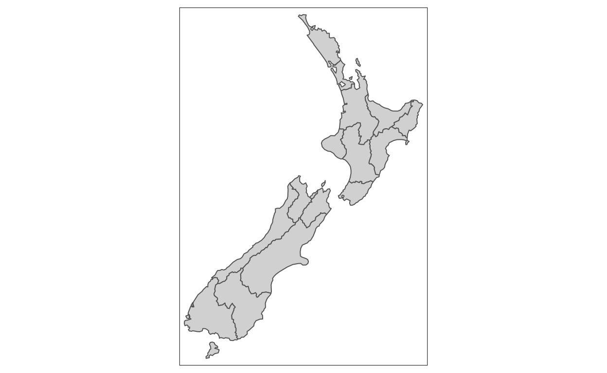
Making a basic map of New Zealand with tmap. The New Zealand object comes from the sf data

tm_polygons() combines both tm_fill() and tm_borders() so map_nz1 and map_nz2 below are the same.

Show code

map_nz1 <- tm_shape(nz) +
  tm_fill() + 
  tm_borders() 

map_nz2 <- tm_shape(nz) + tm_polygons()
map_nz2

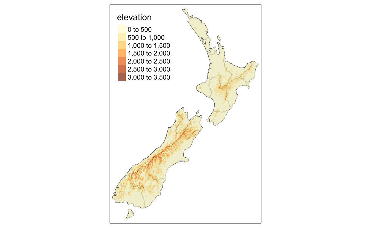
Combining multiple layers

tm_raster() plots a raster layer and the argument alpha is the transparency of that layer

Show code

map_nz3 <- map_nz2 + tm_shape(nz_elev) +
  tm_raster(alpha = 0.7) 
map_nz3

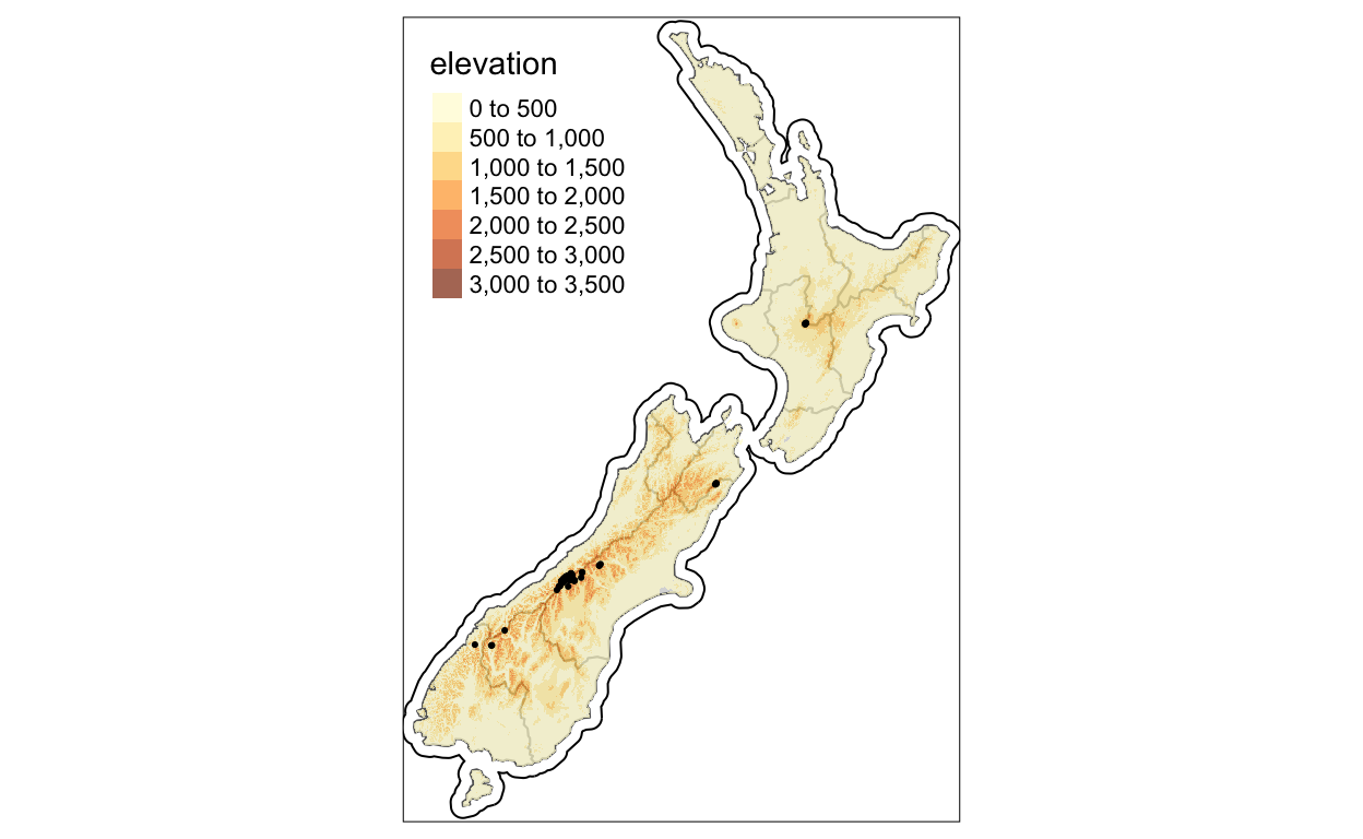
New Zealand water addition

Show code

nz_water <- st_union(nz) %>% #returns a single geometry with resolved boundaries
  st_buffer(22200) %>% #computes a buffer around this geometry
  st_cast(to = "LINESTRING") #cast geometry to another type

map_nz4 <- map_nz3 + 
  tm_shape(nz_water) + tm_lines()
map_nz4

Adding the height element to the map of New Zealand

Show code

map_nz5 <- map_nz4 + 
  tm_shape(nz_height) + tm_dots()

map_nz5

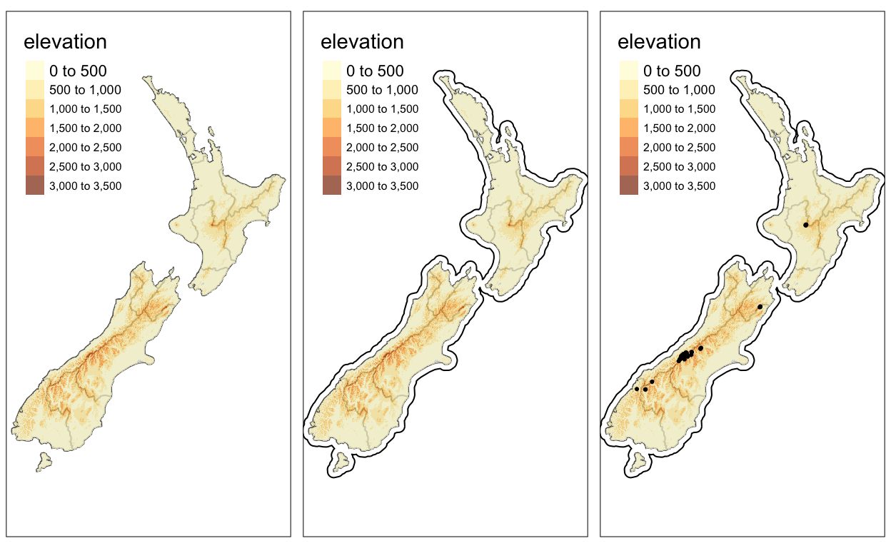
To combine different maps using tmap in a similar way as you would use patchwork in ggplot you do the following:

Show code

tmap_arrange(map_nz3, map_nz4, map_nz5)

tmap aesthetics

The common aesthetics for fill and border layers are color col , transparency alpha , line width lwd and line typelty.

Show code

map1 <- tm_shape(nz) + tm_fill(col = "green")
map2 <- tm_shape(nz) + tm_fill(col = "red", alpha = 0.5)
map3 <- tm_shape(nz) + tm_borders(col = "darkgrey")
map4 <- tm_shape(nz) + tm_borders(lwd = 2)
map5 <- tm_shape(nz) + tm_borders(lty = 3)
map6 <- tm_shape(nz) + tm_fill(col = "green", alpha = 0.5) +
  tm_borders(col = "darkgrey", lwd = 2, lty = 3)
tmap_arrange(map1, map2, map3, map4, map5, map6)

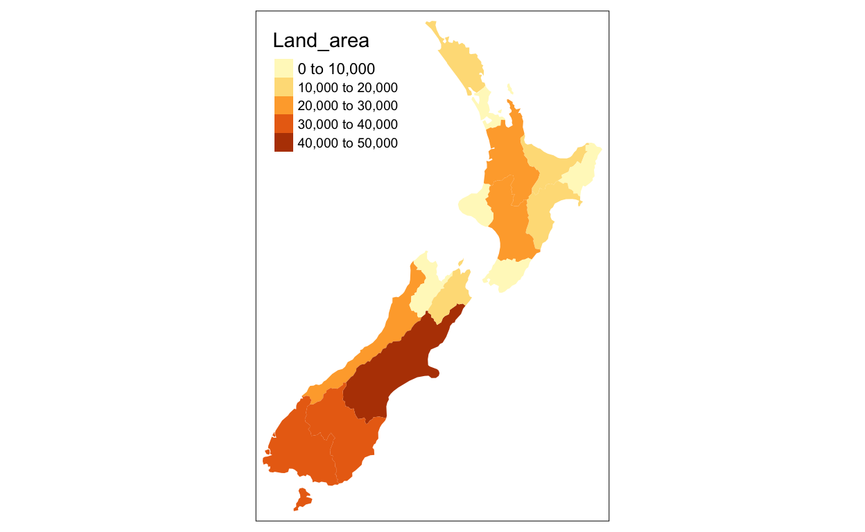
You cannot use a column name in tmap like you can in R to set the aesthetic of a variable like color, but instead you have to put it in quotations. You can treat plot the same way as you would R though. Hopefully, I am understanding this correctly.

Show code

# tm_shape(nz) + tm_fill(col = nz$Land_area) This line fails
plot(st_geometry(nz), col = nz$Land_area) # This works because plot has the same functionality as R

Show code

tm_shape(nz) + tm_fill(col = "Land_area") #The color aesthetic has to be in quotes here 

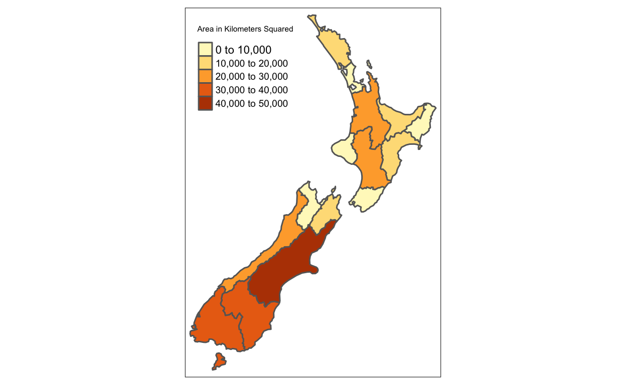
To add a title in the legend of the aesthetic you are using, you define this in the same place as you define the aesthetic. expression() is used in the commented seciton below to add the special script for the squared kilometers. If you do not need fancy text, you can just put your title in quotes.

Show code

#legend_title = expression("Area (km"^2*")") 
legend_title = "Area in Kilometers Squared"
map_nza = tm_shape(nz) +
  tm_fill(col = "Land_area", title = legend_title) + tm_borders(lwd = 1.5)
map_nza

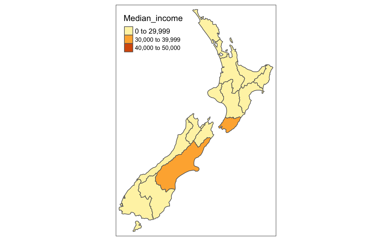
Color Settings

Show code

tm_shape(nz) + tm_polygons(col = "Median_income")

Show code

breaks = c(0, 3, 4, 5) * 10000
tm_shape(nz) + tm_polygons(col = "Median_income", breaks = breaks)

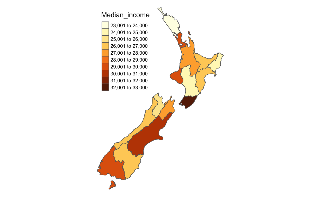
Show code

tm_shape(nz) + tm_polygons(col = "Median_income", n = 10)

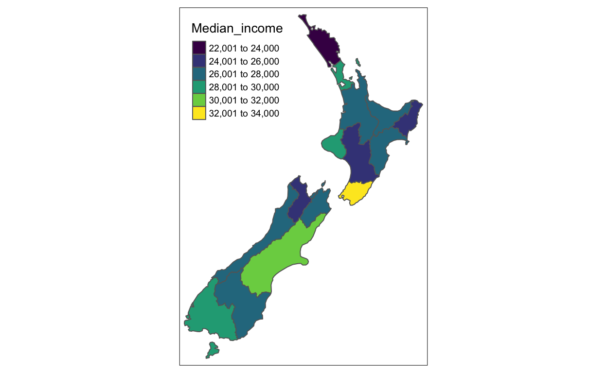
Show code

tm_shape(nz) + tm_polygons(col = "Median_income", palette = "viridis")

This is all the map work I’ve done for the day! Stay tuned, maybe there will be more.